Applets:Bessel Functions of the First Kind: Unterschied zwischen den Versionen
| Zeile 114: | Zeile 114: | ||
Such a window function provides, for example, the Kaiser–Bessel–window ⇒ see section [[Signaldarstellung/Spektralanalyse#Spezielle_Fensterfunktionen|Special Window Functions]]. Its time-discrete Fenser function reads with the Bessel function zero order ⇒ ${\rm J}_0(x)$, the parameter $\alpha=3.5$ and the window length $N$: | Such a window function provides, for example, the Kaiser–Bessel–window ⇒ see section [[Signaldarstellung/Spektralanalyse#Spezielle_Fensterfunktionen|Special Window Functions]]. Its time-discrete Fenser function reads with the Bessel function zero order ⇒ ${\rm J}_0(x)$, the parameter $\alpha=3.5$ and the window length $N$: | ||
:$$w_\nu = \frac{ {\rm J}_0\big(\pi \cdot \alpha \cdot \sqrt{1 - (2\nu/N)^2}\big)}{ {\rm J}_0\big(\pi \cdot \alpha \big)}.$$ | :$$w_\nu = \frac{ {\rm J}_0\big(\pi \cdot \alpha \cdot \sqrt{1 - (2\nu/N)^2}\big)}{ {\rm J}_0\big(\pi \cdot \alpha \big)}.$$ | ||
| − | + | On the page [[Signaldarstellung/Spektralanalyse#G.C3.BCtekriterien_von_Fensterfunktionen|Quality Criteria of Window Functions]] and other the characteristics of the Kaiser-Bessel-window are given: | |
| − | * | + | *Conveniently, the large is „minimum distance between the main lobe and side lobes” and the desired small „maximum scaling error”. |
| − | * | + | *Due to the very large „equivalent noise width” the Kaiser-Bessel window cuts in the main comparison criterion „maximum process loss” but worse off than the established Hamming– and Hanning–windows.}} |
{{GraueBox|TEXT= | {{GraueBox|TEXT= | ||
| − | $\text{ | + | $\text{Example (D):} \hspace{0.5cm} \text{Rice-Fading channel model}$ |
| − | + | The [[Mobile_Kommunikation/Wahrscheinlichkeitsdichte_des_Rayleigh%E2%80%93Fadings#Allgemeine_Beschreibung_des_Mobilfunkkanals| Rayleigh - Distribution]] describes the mobile channel assuming that there is no direct path, and thus the multiplicative factor $z(t) = x(t) + {\rm j} \cdot y(t)$ is solely diffuse composed of scattered components. | |
| − | + | In the case of a direct component (English: <i>Line of Sight</i>, LoS) in the model for the mean-free Gaussian processes $x(t)$ and $y(t)$ one has to add equal components $x_0$ and/or $y_0$ : | |
| − | [[Datei:P ID2126 Mob T 1 4 S1 v3.png|right|frame|Rice-Fading | + | [[Datei:P ID2126 Mob T 1 4 S1 v3.png|right|frame|Rice-Fading channel model|class=fit]] |
$$\hspace{0.2cm}x(t) \hspace{0.1cm} \Rightarrow \hspace{0.1cm} x(t) +x_0 \hspace{0.05cm}, \hspace{0.2cm} y(t) \hspace{0.1cm} \Rightarrow \hspace{0.1cm} y(t) +y_0\hspace{0.05cm},$$ | $$\hspace{0.2cm}x(t) \hspace{0.1cm} \Rightarrow \hspace{0.1cm} x(t) +x_0 \hspace{0.05cm}, \hspace{0.2cm} y(t) \hspace{0.1cm} \Rightarrow \hspace{0.1cm} y(t) +y_0\hspace{0.05cm},$$ | ||
| Zeile 132: | Zeile 132: | ||
z_0 = x_0 + {\rm j} \cdot y_0\hspace{0.05cm}.$$ | z_0 = x_0 + {\rm j} \cdot y_0\hspace{0.05cm}.$$ | ||
| − | + | The graph shows the ''Rice–Fading–Channel model''. It can be summarized as follows: | |
| − | * | + | *The real part $x(t)$ is Gaussianized with mean $x_0$ and variance $\sigma ^2$. |
| − | * | + | *The imaginary part $y(t)$ is also Gaussian (mean $y_0$, equal variance $\sigma ^2$) and independent of $x(t)$.<br> |
| − | * | + | *For $z_0 \ne 0$, the amount $\vert z(t)\vert$ rice is distributed, from which the term „<i>Rice–Fading</i>” arises. |
| − | * | + | *To simplify the notation, we set $\vert z(t)\vert = a(t)$. For $a < 0$ , the amounts - WDF are $f_a(a) \equiv 0$, for $a \ge 0$ the following equation holds, where ${\rm I_0}(x)$ is the <i>modified Besselfunktion</i> zeroth order denotes: |
| − | :$$f_a(a) = \frac{a}{\sigma^2} \cdot {\rm e}^{ - (a^2 + \vert z_0 \vert ^2)/(2\sigma^2)} \cdot {\rm I}_0 \left [ \frac{a \cdot \vert z_0 \vert}{\sigma^2} \right ] \hspace{0.5cm}\text{ | + | :$$f_a(a) = \frac{a}{\sigma^2} \cdot {\rm e}^{ - (a^2 + \vert z_0 \vert ^2)/(2\sigma^2)} \cdot {\rm I}_0 \left [ \frac{a \cdot \vert z_0 \vert}{\sigma^2} \right ] \hspace{0.5cm}\text{with}\hspace{0.5cm}{\rm I }_0 (u) = {\rm J }_0 ({\rm j} \cdot u) = |
\sum_{k = 0}^{\infty} \frac{ (u/2)^{2k} }{k! \cdot \Gamma (k+1)} | \sum_{k = 0}^{\infty} \frac{ (u/2)^{2k} }{k! \cdot \Gamma (k+1)} | ||
\hspace{0.05cm}.$$ | \hspace{0.05cm}.$$ | ||
| − | * | + | *Between the modified Bessel function and the traditional Bessel function ${\rm I_0}(x)$ – each first type – So the connection exists ${\rm I }_0 (u) = {\rm J }_0 ({\rm j} \cdot u)$.}} |
{{GraueBox|TEXT= | {{GraueBox|TEXT= | ||
| − | $\text{ | + | $\text{Example (E):} \hspace{0.5cm} \text{Analysis of the frequency spectrum of frequency modulated signals}$ |
| − | + | $\text{Example (B)}$ has already shown that the angle modulation of a harmonic oscillation of the frequency $f_{\rm N}$ leads to a line spectrum. The spectral lines are around the carrier frequency $f_{\rm T}$ bei $f_{\rm T} + n \cdot f_{\rm N}$ with $n \in \{ \ \text{...}, -2, -1, \ 0, +1, +2, \text{...} \ \}$. The weights of the Dirac lines are ${\rm J }_n(\eta)$, depending on the modulation index $\eta$. | |
| − | [[Datei:P_ID1095__Mod_T_3_2_S4_neu.png|center|frame| | + | [[Datei:P_ID1095__Mod_T_3_2_S4_neu.png|center|frame|Discrete spectra with phase modulation (left) and frequency modulation (right)]] |
| − | + | The graph shows the magnitude spectrum $\vert S_{\rm +}(f) \vert$ of the phase modulation (PM) and frequency modulation (FM) analytical signal, two different forms of angle modulation (WM). Bessellines with values less than $0.03$ are neglected in both cases. | |
| − | + | For the upper half of the image, the modulator parameters are chosen so that for each $f_{\rm N} = 5 \ \rm kHz$ here is a Bessel spectrum with the modulation index $η = 1.5$. Disregarding the phase relationships, the same spectra and the same signals result for both systems. | |
| − | + | The lower graphics are valid for the same message frequency $f_{\rm N} = 3 \ \rm kHz$. One notices: | |
| − | * | + | *In phase modulation, the spectral function is narrower than $f_{\rm N} = 5 \ \rm kHz$, because the distance of the Bessel lines is now only $3 \ \rm kHz$. Since the modulation index of PM is independent of $f_{\rm N}$, the same bessel weights result as in $f_{\rm N} = 5 \ \rm kHz$. |
| − | * | + | *Also in the frequency modulation, the Bessel lines now appear at a distance of $3 \ \rm kHz$. However, since FM has a modulation index inversely proportional to $f_{\rm N}$, there is now much more Besselline lines than in the upper right (for $η = 1.5$ valid) chart due to the larger modulation index $η = 2.5$.}} |
Version vom 21. August 2018, 23:02 Uhr
Inhaltsverzeichnis
Applet Description
This applet allows the calculation and graphical representation of the Bessel functions of the first kind and $n$–th order according to the series representation:
- $${\rm J}_n (x) = \sum\limits_{k=0}^{\infty}\frac{(-1)^k \cdot (x/2)^{n \hspace{0.05cm} + \hspace{0.05cm} 2 \hspace{0.02cm}\cdot \hspace{0.05cm}k}}{k! \cdot (n+k)!} \hspace{0.05cm}.$$
- Graphically represented, the functions ${\rm J}_n (x)$ for the order $n=0$ to $n=9$ can become different colors.
- The left-hand output provides the function values ${\rm J}_0 (x = x_1)$, ... , ${\rm J}_9 (x = x_1)$ for a slider-settable value $x_1$ in the range $0 \le x_1 \le 15$ with increment $0.5$.
- The right hand side returns the function values ${\rm J}_0 (x = x_2)$, ... , ${\rm J}_9 (x = x_2)$ for a slider-settable value $x_2$ (same range and value) Increment as on the left).
Theoretical Background
General Information about the Bessel Functions
Bessel functions (or cylinder functions) are solutions of the Bessel differential equation of the form
- $$x^2 \cdot \frac{ {\rm d}^2}{{\rm d}x^2}\ {\rm J}_n (x) \ + \ x \cdot \frac{ {\rm d}}{{\rm d}x}\ {\rm J}_n (x) \ + \ (x^2 - n^2) \cdot {\rm J}_n (x)= 0. $$
This is an ordinary second-order linear differential equation. The parameter $ n $ is usually integer, as in this program. These mathematical functions, which were introduced in 1844 by Friedrich Wilhelm Bessel, can also be represented in closed form as integrals:
- $${\rm J}_n (x) = \frac{1}{2\pi}\cdot \int_{-\pi}^{+\pi} {{\rm e}^{\hspace{0.05cm}{\rm j}\hspace{0.05cm}\cdot \hspace{0.05cm}[\hspace{0.05cm}x \hspace{0.05cm}\cdot \hspace{0.05cm}\sin(\alpha) -\hspace{0.05cm} n \hspace{0.05cm}\cdot \hspace{0.05cm}\alpha \hspace{0.05cm}]}}\hspace{0.1cm}{\rm d}\alpha \hspace{0.05cm}.$$
The functions ${\rm J}_n (x)$ belong to the class of Bessel functions of the first kind (German: Besselfunktionen erster Art). The parameter $n$ is called the Order.
Annotation: There are a number of modifications of the Bessel functions, including the second-order Bessel functions named ${\rm Y}_n (x)$. For integer $n$, ${\rm Y}_n (x)$ can be replaced by ${\rm J}_n (x)$–functions. However, in this applet, only the first-order Bessel functions are ⇒ ${\rm J}_n (x)$ is considered.
Properties of the Bessel Functions
$\text{Property (A):}$ If the function values for $n = 0$ and $n = 1$ are known, then the Bessel function for $n ≥ 2$ can be determined iteratively:
- $${\rm J}_n (x) ={2 \cdot (n-1)}/{x} \cdot {\rm J}_{n-1} (x) - {\rm J}_{n-2} (x) \hspace{0.05cm}.$$
$\text{Example (A):}$ Consider ${\rm J}_0 (x = 2) = 0.22389$ and ${\rm J}_1 (x= 2) = 0.57672$. From this it can be calculated iteratively:
- $${\rm J}_2 (x= 2) ={2 \cdot 1}/{2} \cdot {\rm J}_{1} (x= 2) - {\rm J}_{0} (x= 2) = 0.57672 - 0.22389 = \hspace{0.15cm}\underline{0.35283}\hspace{0.05cm},$$
- $${\rm J}_3 (x= 2) ={2 \cdot 2}/{2} \cdot {\rm J}_{2} (x= 2) - {\rm J}_{1} (x= 2) = 2 \cdot 0.35283 - 0.57672 = \hspace{0.15cm}\underline{0.12894}\hspace{0.05cm},$$
- $${\rm J}_4 (x= 2) ={2 \cdot 3}/{2} \cdot {\rm J}_{3} (x= 2) - {\rm J}_{2} (x= 2) = 3 \cdot 0.12894 - 0.35283 = \hspace{0.15cm}\underline{0.03400}\hspace{0.05cm}.$$
$\text{Property (B):}$ The symmetry relationship applies ${\rm J}_{–n}(x) = (–1)^n · {\rm J}_n(x)$:
- $${\rm J}_{-1}(x) = - {\rm J}_{1}(x), \hspace{0.3cm}{\rm J}_{-2}(x) = {\rm J}_{2}(x), \hspace{0.3cm}{\rm J}_{-3}(x) = - {\rm J}_{3}(x).$$
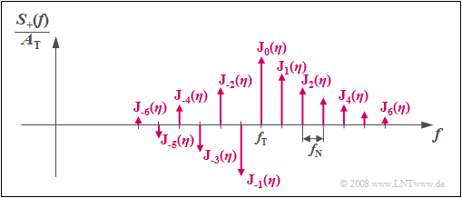
$\text{Example (B):}$ For the spectrum of the analytic signal, in phase modulation of a sinusoidal signal:
- $$S_{\rm +}(f) = A_{\rm T} \cdot \sum_{n = - \infty}^{+\infty}{\rm J}_n (\eta) \cdot \delta \big[f - (f_{\rm T}+ n \cdot f_{\rm N})\big]\hspace{0.05cm}.$$
Denote this
- $f_{\rm T}$ the carrier frequency,
- $f_{\rm N}$ the message frequency,
- $A_{\rm T}$ the carrier amplitude.
The parameter of the Bessel functions in this application is the modulation index $\eta$.
Based on the graphic, the following statements are possible:
- Here $S_+(f)$ consists of an infinite number of discrete lines at a distance of $f_{\rm N}$.
- It is thus in principle infinitely extended.
- The weights of the spectral lines at $f_{\rm T} + n · f_{\rm N}$ ($n$ integer) are determined by the modulation index $η$ over the Bessel functions ${\rm J}_n(η)$.
- The spectral lines are real in the case of a sinusoidal source signal and a cosinusoidal carrier and symmetric about $f_{\rm T}$ for even $n$.
- For odd $n$ , a sign change according to the $\text{Property (B)}$ has to be considered.
- The phase modulation of another phase oscillation of source and / or carrier signal provides the same magnitude spectrum.
Applications of the Bessel Functions
The applications of the Bessel functions in nature–and engineering are diverse and play an important role in physics, for example:
- Examination of natural vibrations of cylindrical resonators,
- Solution of the radial Schrödinger-equation,
- Sound pressure amplitudes of low-viscosity rotational flows,
- Heat conduction in cylindrical bodies,
- Scattering problem of a grid,
- Dynamics of oscillating bodies,
- Angular resolution.
The Bessel functions are counted among the special functions because of their many applications in mathematical physics.
In the following, we restrict ourselves to a few areas that are addressed in our tutorial $\rm LNTwww$.
In the English original Electromagnetic waves in a cylindrical waveguide Pressure amplitudes of inviscid rotational flows Heat conduction in a cylindrical object Modes of vibration of a thin circular (or annular) acoustic membrane (such as a drum or other membranophone) Diffusion problems on a lattice Solutions to the radial Schrödinger equation (in spherical and cylindrical coordinates) for a free particle Solving for patterns of acoustical radiation Frequency-dependent friction in circular pipelines Dynamics of floating bodies Angular resolution The Ende
$\text{Example (C):} \hspace{0.5cm} \text{Use in spectral analysis} \ \Rightarrow \ \text{Kaiser-Bessel filter}$
The spectral leakage effect is the falsification of the spectrum of a periodic and hence temporally unlimited signal due to the implicit time limitation of the discrete Fourier transform (DFT). This will be done, for example, by a spectrum analyzer
- in the time signal not existing frequency components simulated, and / or
- actually existing spectral components are obscured by sidelobes.
The task of the spectral analysis is to limit the influence of the spectral leakage effect by providing suitable window functions.
Such a window function provides, for example, the Kaiser–Bessel–window ⇒ see section Special Window Functions. Its time-discrete Fenser function reads with the Bessel function zero order ⇒ ${\rm J}_0(x)$, the parameter $\alpha=3.5$ and the window length $N$:
- $$w_\nu = \frac{ {\rm J}_0\big(\pi \cdot \alpha \cdot \sqrt{1 - (2\nu/N)^2}\big)}{ {\rm J}_0\big(\pi \cdot \alpha \big)}.$$
On the page Quality Criteria of Window Functions and other the characteristics of the Kaiser-Bessel-window are given:
- Conveniently, the large is „minimum distance between the main lobe and side lobes” and the desired small „maximum scaling error”.
- Due to the very large „equivalent noise width” the Kaiser-Bessel window cuts in the main comparison criterion „maximum process loss” but worse off than the established Hamming– and Hanning–windows.
$\text{Example (D):} \hspace{0.5cm} \text{Rice-Fading channel model}$
The Rayleigh - Distribution describes the mobile channel assuming that there is no direct path, and thus the multiplicative factor $z(t) = x(t) + {\rm j} \cdot y(t)$ is solely diffuse composed of scattered components.
In the case of a direct component (English: Line of Sight, LoS) in the model for the mean-free Gaussian processes $x(t)$ and $y(t)$ one has to add equal components $x_0$ and/or $y_0$ :
$$\hspace{0.2cm}x(t) \hspace{0.1cm} \Rightarrow \hspace{0.1cm} x(t) +x_0 \hspace{0.05cm}, \hspace{0.2cm} y(t) \hspace{0.1cm} \Rightarrow \hspace{0.1cm} y(t) +y_0\hspace{0.05cm},$$
$$\hspace{0.2cm}z(t) = x(t) + {\rm j} \cdot y(t) \hspace{0.1cm} \Rightarrow \hspace{0.1cm} z(t) +z_0 \hspace{0.05cm},\hspace{0.2cm} z_0 = x_0 + {\rm j} \cdot y_0\hspace{0.05cm}.$$
The graph shows the Rice–Fading–Channel model. It can be summarized as follows:
- The real part $x(t)$ is Gaussianized with mean $x_0$ and variance $\sigma ^2$.
- The imaginary part $y(t)$ is also Gaussian (mean $y_0$, equal variance $\sigma ^2$) and independent of $x(t)$.
- For $z_0 \ne 0$, the amount $\vert z(t)\vert$ rice is distributed, from which the term „Rice–Fading” arises.
- To simplify the notation, we set $\vert z(t)\vert = a(t)$. For $a < 0$ , the amounts - WDF are $f_a(a) \equiv 0$, for $a \ge 0$ the following equation holds, where ${\rm I_0}(x)$ is the modified Besselfunktion zeroth order denotes:
- $$f_a(a) = \frac{a}{\sigma^2} \cdot {\rm e}^{ - (a^2 + \vert z_0 \vert ^2)/(2\sigma^2)} \cdot {\rm I}_0 \left [ \frac{a \cdot \vert z_0 \vert}{\sigma^2} \right ] \hspace{0.5cm}\text{with}\hspace{0.5cm}{\rm I }_0 (u) = {\rm J }_0 ({\rm j} \cdot u) = \sum_{k = 0}^{\infty} \frac{ (u/2)^{2k} }{k! \cdot \Gamma (k+1)} \hspace{0.05cm}.$$
- Between the modified Bessel function and the traditional Bessel function ${\rm I_0}(x)$ – each first type – So the connection exists ${\rm I }_0 (u) = {\rm J }_0 ({\rm j} \cdot u)$.
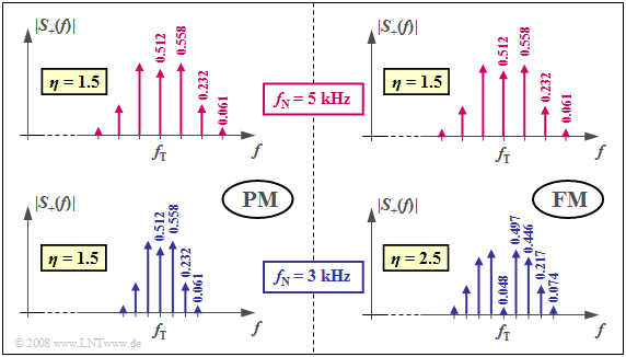
$\text{Example (E):} \hspace{0.5cm} \text{Analysis of the frequency spectrum of frequency modulated signals}$
$\text{Example (B)}$ has already shown that the angle modulation of a harmonic oscillation of the frequency $f_{\rm N}$ leads to a line spectrum. The spectral lines are around the carrier frequency $f_{\rm T}$ bei $f_{\rm T} + n \cdot f_{\rm N}$ with $n \in \{ \ \text{...}, -2, -1, \ 0, +1, +2, \text{...} \ \}$. The weights of the Dirac lines are ${\rm J }_n(\eta)$, depending on the modulation index $\eta$.
The graph shows the magnitude spectrum $\vert S_{\rm +}(f) \vert$ of the phase modulation (PM) and frequency modulation (FM) analytical signal, two different forms of angle modulation (WM). Bessellines with values less than $0.03$ are neglected in both cases.
For the upper half of the image, the modulator parameters are chosen so that for each $f_{\rm N} = 5 \ \rm kHz$ here is a Bessel spectrum with the modulation index $η = 1.5$. Disregarding the phase relationships, the same spectra and the same signals result for both systems.
The lower graphics are valid for the same message frequency $f_{\rm N} = 3 \ \rm kHz$. One notices:
- In phase modulation, the spectral function is narrower than $f_{\rm N} = 5 \ \rm kHz$, because the distance of the Bessel lines is now only $3 \ \rm kHz$. Since the modulation index of PM is independent of $f_{\rm N}$, the same bessel weights result as in $f_{\rm N} = 5 \ \rm kHz$.
- Also in the frequency modulation, the Bessel lines now appear at a distance of $3 \ \rm kHz$. However, since FM has a modulation index inversely proportional to $f_{\rm N}$, there is now much more Besselline lines than in the upper right (for $η = 1.5$ valid) chart due to the larger modulation index $η = 2.5$.
Das folgende Kapitel muss noch angepasst werden!
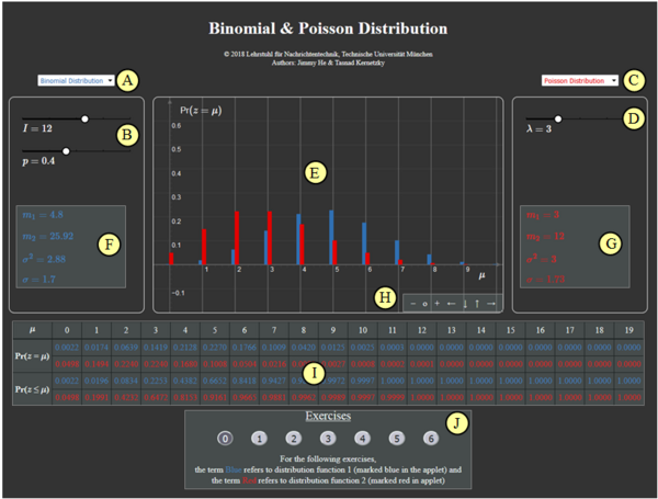
Zur Handhabung des Applets
(A) Vorauswahl für blauen Parametersatz
(B) Parametereingabe $I$ und $p$ per Slider
(C) Vorauswahl für roten Parametersatz
(D) Parametereingabe $\lambda$ per Slider
(E) Graphische Darstellung der Verteilungen
(F) Momentenausgabe für blauen Parametersatz
(G) Momentenausgabe für roten Parametersatz
(H) Variation der grafischen Darstellung
$\hspace{1.5cm}$„$+$” (Vergrößern),
$\hspace{1.5cm}$ „$-$” (Verkleinern)
$\hspace{1.5cm}$ „$\rm o$” (Zurücksetzen)
$\hspace{1.5cm}$ „$\leftarrow$” (Verschieben nach links), usw.
( I ) Ausgabe von ${\rm Pr} (z = \mu)$ und ${\rm Pr} (z \le \mu)$
(J) Bereich für die Versuchsdurchführung
Andere Möglichkeiten zur Variation der grafischen Darstellung:
- Gedrückte Shifttaste und Scrollen: Zoomen im Koordinatensystem,
- Gedrückte Shifttaste und linke Maustaste: Verschieben des Koordinatensystems.
Über die Autoren
Dieses interaktive Berechnungstool wurde am Lehrstuhl für Nachrichtentechnik der Technischen Universität München konzipiert und realisiert.
- Die erste Version wurde 2006 von Markus Elsberger und Slim Lamine im Rahmen von Abschlussarbeiten mit „FlashMX–Actionscript” erstellt (Betreuer: Günter Söder).
- 2018 wurde das Programm von Xiaohan Liu (Bachelorarbeit, Betreuer: Tasnád Kernetzky ) auf „HTML5” umgesetzt.


