(13 dazwischenliegende Versionen von 4 Benutzern werden nicht angezeigt)
Zeile 2:
Zeile 2:
}}
}}
[[Datei:P_ID2122__Mob_A_1_2.png|right|frame|PDF of lognormal fading]]
[[Datei:EN_Mob_A1_2.png|right|frame|PDF of lognormal fading]]
We consider a mobile radio cell in an urban area and a vehicle that is approximately at a fixed distance $d_0$ from the base station. For example, it moves on an arc around the base station.
We consider a mobile radio cell in an urban area and a vehicle that is approximately at a fixed distance $d_0$ from the base station. For example, it moves on an arc around the base station.
Thus the total path loss can be described by the following equation:
Thus the total path loss can be described by the following equation:
* Or use the interaction module provided by $\rm LNTwww$ [[Applets:Komplementäre_Gaußsche_Fehlerfunktionen|Komplementäre Gaußsche Fehlerfunktionen]].
* Or use the interaction module provided by $\rm LNTwww$ [[Applets:Komplementäre_Gaußsche_Fehlerfunktionen_(neues_Applet)|Komplementäre Gaußsche Fehlerfunktionen]].
Zeile 59:
Zeile 58:
'''(1)''' The correct answer is <u>YES</u>:
'''(1)''' The correct answer is <u>YES</u>:
*From the $\rm dB$–value $V_0 = 80 \ \rm dB$ follows the absolute (linear) value $K_0 = 10^8$. Thus the received power is
*From the $\rm dB$–value $V_0 = 80 \ \rm dB$ follows the absolute (linear) value $K_0 = 10^8$. Thus the received power is
*Only the limit value $–80 \ \rm dBm$ is required.
*Only the limit value $–80 \ \rm dBm$ is required.
Zeile 69:
Zeile 67:
'''(2)''' Lognormal–Fading with $\sigma_{\rm S} = 0 \ \rm dB$ is equivalent to a constant receive reading $P_{\rm E}$.
'''(2)''' Lognormal–Fading with $\sigma_{\rm S} = 0 \ \rm dB$ is equivalent to a constant receive power $P_{\rm E}$.
*Compared to the subtask '''(1)'' this is $m_{\rm S} = 20 \ \ \rm dB$ smaller ⇒ $P_{\rm E} = \ –60 \ \ \rm dBm$.
*Compared to the subtask '''(1)'' this is $m_{\rm S} = 20 \ \ \rm dB$ smaller ⇒ $P_{\rm E} = \ –60 \ \ \rm dBm$.
*But it is still greater than the specified limit value ($–80 \ \rm dBm$).
*But it is still greater than the specified limit value ($–80 \ \rm dBm$).
*It follows: The system is (almost) <u>100% functional</u>. „Fast” because with a Gaussian random quantity there is always a (small) residual uncertainty.
*It follows: The system is (almost) <u>100% functional</u>. „Almost” because with a Gaussian random quantity there is always a (small) residual uncertainty.
Zeile 79:
Zeile 77:
*The variable portion $V_{\rm S}$ must therefore not be greater than $20 \ \rm dB$.
*The variable portion $V_{\rm S}$ must therefore not be greater than $20 \ \rm dB$.
*So it follows:
*So it follows:
$${\rm Pr}({\rm "System\hspace{0.15cm} does not work\hspace{0.15cm}"})= {\rm Q}\left ( \frac{20\,\,{\rm dB}}}{\sigma_{\rm S} = 10\,{\rm dB}\right )
[[File:P_ID2187__Mob_A_1_2c_v1.png|right|frame|loss due to lognormal fading]]
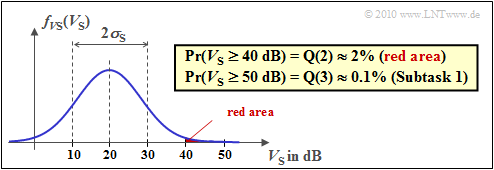
The graphic illustrates the result.
The graphic illustrates the result.
*The probability density $f_{\rm VS}(V_{\rm S})$ of the path loss due to shadowing (Longnormal–Fading) is shown here.
*The probability density $f_{\rm VS}(V_{\rm S})$ of the path loss due to shadowing (Longnormal–Fading) is shown here.
*Die Wahrscheinlichkeit, dass das System ausfällt, ist rot markiert:
<br clear=all>
'''(4)''' Aus der Verfügbarkeitswahrscheinlichkeit $99.9 \%$ folgt die Ausfallwahrscheinlichkeit $10^{\rm –3} \approx \ {\rm Q}(3)$.
*Verringert man den entfernungsabhängigen Pfadverlust $V_0$ um $10 \ \rm dB$ auf $\underline {70 \ \rm dB}$, so kommt es erst dann zu einem Ausfall, wenn $V_{\rm S} ≥ 50 \ \rm dB$ ist.
*Damit wäre genau die geforderte Zuverlässigkeit erreicht, wie die folgende Rechnung zeigt:
*The probability that the system will fail is marked in red:
*The probability that the system will fail is marked in red.
<br clear=all>
<br clear=all>
'''(4)''' From the availability probability $99.9 \%$ follows the default probability $10^{\rm –3} \approx \ {\rm Q}(3)$.
'''(4)''' From the availability probability $99.9 \%$ follows the failure probability $10^{\rm –3} \approx \ {\rm Q}(3)$.
*If the distance-dependent path loss $V_0$ is reduced by $10 \ \ \rm dB$ to $\underline {70 \ \rm dB}$, a failure will only occur when $V_{\rm S} ≥ 50 \ \ \rm dB$.
*If the distance-dependent path loss $V_0$ is reduced by $10 \ \ \rm dB$ to $\underline {70 \ \rm dB}$, a failure will only occur when $V_{\rm S} ≥ 50 \ \ \rm dB$.
*This would achieve exactly the required reliability, as the following calculation shows:
*This would achieve exactly the required reliability, as the following calculation shows:
$${\rm Pr}({\rm "System\hspace{0.15cm} does not work\hspace{0.15cm}"})=
We consider a mobile radio cell in an urban area and a vehicle that is approximately at a fixed distance $d_0$ from the base station. For example, it moves on an arc around the base station.
Thus the total path loss can be described by the following equation:
The probability density $f_{\rm VS}(V_{\rm S})$ of the path loss due to shadowing (Longnormal–Fading) is shown here.
The probability that the system will fail is marked in red.
(4) From the availability probability $99.9 \%$ follows the failure probability $10^{\rm –3} \approx \ {\rm Q}(3)$.
If the distance-dependent path loss $V_0$ is reduced by $10 \ \ \rm dB$ to $\underline {70 \ \rm dB}$, a failure will only occur when $V_{\rm S} ≥ 50 \ \ \rm dB$.
This would achieve exactly the required reliability, as the following calculation shows: