Linear Distortions of Periodic Signals
Inhaltsverzeichnis
Applet description
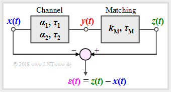
This applet illustrates the effects of linear distortions (attenuation distortions and phase distortions) with
- the input signal x(t) ⇒ power Px:
- x(t)=x1(t)+x2(t)=A1⋅cos(2πf1⋅t−φ1)+A2⋅cos(2πf2⋅t−φ2),
- the output signal y(t) ⇒ power Py:
- y(t)=α1⋅x1(t−τ1)+α2⋅x2(t−τ2),
- the matching output signal z(t) ⇒ power Pz:
- z(t)=kM⋅y(t−τM)+α2⋅x2(t−τ2),
- the difference signal ε(t)=z(t)−x(t) ⇒ power Pε.
The next block in the above model is Matching: The output signal y(t) is adjusted in amplitude and phase with uniform quantities kM and τM for all frequencies which means that this is not a frequency-dependent distortion. Using the signal z(t), a differentiation can be made between:
- attenuation distortion and frequency–independant attenuation, as well as
- phase distortion and pure frequency–independant delay.
The Distortion Power PD is used to measure the strength of the linear distortion and is defined as:
- PD=minkM, τMPε.
Theoretical background
Distortions refer to generally unwanted alterations of a message signal through a transmission system. Together with the strong stochastic effects (noise, crosstalk, etc.), they are a crucial limitation for the quality and rate of transmission.
Just as the intensity of noise can be assessed through
- the Noise Power PN and
- the Signal–to–Noise Ratio (SNR) ρN,
distortions can be quantified through
- the Distortion Power PD and
- the Signal–to–Distortion Ratio (SDR)
- ρD=Signal PowerDistortion Power=PxPD.
Linear and nonlinear distortions
A distinction is made between linear and nonlinear distortions:
- Nonlinear distortions occur, if at all times t the nonlinear correlation y=g(x)≠const.⋅x exists between the signal values x=x(t) at the input and y=y(t) at the output, whereby y=g(x) is defined as the system's nonlinear characteristic. By creating a cosine signal at the input with frequency f0 the output signal value includes f0 as well as multiple harmonic waves. We conclude that new frequencies arise through nonlinear distortion.
- Linear distortions occur, if the transmission channel is characterized by a frequency response H(f)≠const. Various frequencies are attenuated and delayed differently. Characteristic of this is that although frequencies can disappear (for example, through a Low–pass or a High–pass), no new frequencies can arise.
In this applet only linear distortions are considered.
Description forms for the frequency response
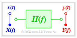
The generally complex valued frequency response can be represented as follows:
- H(f)=|H(f)|⋅e−j⋅b(f)=e−a(f)⋅e−j⋅b(f).
This results in the following description variables:
- The absolute value |H(f)| is called amplitude response and in logarithmic form attenuation function:
- a(f)=−ln|H(f)|inNeper(Np)=−20⋅lg|H(f)|inDecibel(dB).
- The phase function b(f) indicates the negative frequency–dependent angle of H(f) in the complex plane based on the real axis:
- b(f)=−arcH(f)inRadian(rad).
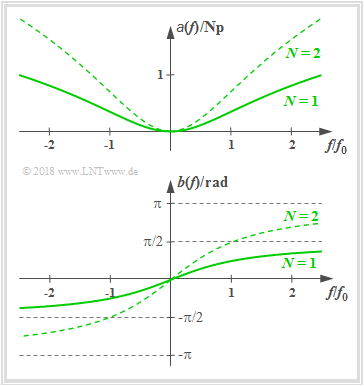
Low–pass of order N
The frequency response of a realizable low pass of order N is:
- H(f)=[11+j⋅f/f0]N.
For example the RC low pass is a first order low–Pass. Consequently we can obtain
- the attenuation function:
- a(f)=N/2⋅ln[1+(f/f0)2],
- the phase function:
- b(f)=N⋅arctan(f/f0),
- the attenuation factor for the frequency f=fi:
- αi=|H(f=fi)|=[1+(fi/f0)2]−N/2
- ⇒x(t)=Ai⋅cos(2πfit)→y(t)=αi⋅Ai⋅cos(2πfit),
- the phase delay for the frequency f=fi:
- τi=b(fi)2πfi=N⋅arctan(fi/f0)2πfi
- ⇒x(t)=Ai⋅cos(2πfit)→y(t)=Ai⋅cos(2πfi(t−τi)).
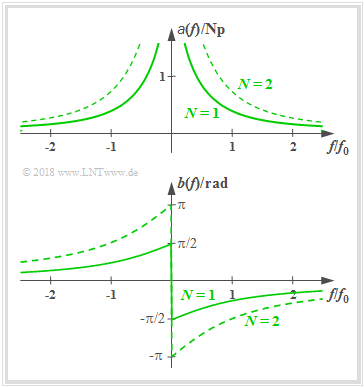
High–pass of order N
The frequency response of a realizable high–pass of order N is:
- H(f)=[j⋅f/f01+j⋅f/f0]N.
For example the LC high pass is a first grade high pass. Consequently we can obtain
- the attenuation function:
- a(f)=N/2⋅ln[1+(f0/f)2],
- the phase function:
- b(f)=−N⋅arctan(f0/f),
- the attenuation factor for the frequency f=fi:
- αi=|H(f=fi)|=[1+(f0/fi)2]−N/2
- ⇒x(t)=Ai⋅cos(2πfit)→y(t)=αi⋅Ai⋅cos(2πfit),
- the phase delay for the frequency f=fi:
- τi=b(fi)2πfi=−N⋅arctan(f0/fi)2πfi
- ⇒x(t)=Ai⋅cos(2πfit)→y(t)=Ai⋅cos(2πfi(t−τi)).
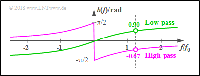
Example: This graphic shows the phase function b(f) with the cut–off frequency f0=1 kHz and order N=1
- of a Low–pass (green curve),
- of a High–pass (violet curve).
The input signal is sinusoidal with frequency fS=1.25 kHz whereby this signal is only turned on at t=0:
- x(t)={0sin(2π⋅fS⋅t)(t<0),(t>0).
The left graphic shows the signal x(t). The dashed line marks the first zero at t=T0=0.8 ms. The other two graphics show the output signals yLP(t) und yHP(t) of low–pass and high–pass, whereby the change in amplitude was balanced in both cases.
- The first zero of the signal yLP(t) after the low–pass is delayed by τLP=0.9/(2π)⋅T0≈0.115 ms compared to the first zero of x(t) ⇒ marked with green arrow, whereby bLP(f/fS=0.9 rad) was considered.
- In contrast, the phase delay of the high–pass is negative: τHP=−0.67/(2π)⋅T0≈−0.085 ms and therefore the first zero of yHP(t) occurs before the dashed line.
- Following this transient response, in both cases the zero crossings again come in the raster of the period duration T0=0.8 ms.
Annotation: The shown signals were created using the interactive applet Causal systems – Laplace transform.
Attenuation distortions and phase distortions
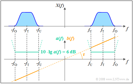
The adjacent figure shows
- the even attenuation function a(f) ⇒ a(−f)=a(f), and
- the uneven function curve b(f) ⇒ b(−f)=−b(−f)
of a non–distorting channel. One notices:
- In a distortion–free system the attenuation function a(f) must be constant betweenfU and fO around the carrier frequency fT, where the input signal exist ⇒ x(t)≠0.
- From the specified constant attenuation value 6 dB follows for the amplitude response |H(f)|=0.5 ⇒ the signal values of all frequencies are thus halved by the system ⇒ no attenuation distortions.
- In addition, in such a system, the phase function b(f) between fU and fO must increase linearly with the frequency. As a result, all frequency components are delayed by the same phase delay τ ⇒ no phase delay.
- The delay τ is fixed by the slope of b(f). The phase function b(f)≡0 would result in a delay–less system ⇒ τ=0.
The following summary considers that in this applet the input signal is always the sum of two harmonic oscillations,
- x(t)=x1(t)+x2(t)=A1⋅cos(2πf1⋅t−φ1)+A2⋅cos(2πf2⋅t−φ2),
and therefor the channel influence is fully described by the attenuation factors α1 and α2 as well as the phase delays τ1 and τ2:
- y(t)=α1⋅x1(t−τ1)+α2⋅x2(t−τ2).
Summary:
- A signal y(t) is only distortion–free compared to x(t) if α1=α2=α and τ1=τ2=τ ⇒ y(t)=α⋅x(t−τ).
- Attenuation distortions occur when α1≠α2. If α1≠α2 and τ1=τ2, then there are exclusively attenuation distortions.
- Phase distortions occur when τ1≠τ2. If τ1≠τ2 and α1=α2, then there are exclusively phase distortions.
Exercises
BlaBla
(1) We set the parameters for the transmitter signal x(t) to A1=0.8 V, A2=0.6 V, f1=0.5 kHz, f2=1.5 kHz, φ1=90∘, φ2=30∘.
- Calculate the signal's cycle duration T0 and power Px. Can you read the value for Px off the applet?
⇒T0=[ greatest common divisor (0.5 kHz, 1.5 kHz)]−1=2.0 ms_;
Px=A21/2+A22/2=0.5 V2_=Pε, if kM=0_ ⇒ z(t)≡0.
(2) Vary φ2 between ±180∘ while assuming the other parameters from (1). How does the value of T0 and Px change?
⇒No changes:T0=2.0 ms;Px=0.5 V2_.
(3) Vary f2 between 0≤f2≤10 kHz while assuming the other parameters from (1). How does the value of Px change?
⇒No changes if f2≠0 oder f2≠f1:Px=0.5 V2_.T0 changes if f2is not a multiple of f1.
If f2=0:Px=A21/2+A22=0.68 V2_.
Iff2=f1:Px=[A1cos(φ1)+A2cos(φ2)]2/2+[A1sin(φ1)+A2sin(φ2)]2/2. Mit φ1=90∘, φ2=30∘:Px=0.74 V2_.
(4) Going by the previous output signal x(t) we set following parameters to: α1=α2=0.5, τ1=τ2=0.5 ms, kM=1 and τM=0 .
- Are there linear distortions? Calculate the reception power Py and the power Pε of the differential signal ε(t)=z(t)−x(t)
⇒y(t)=0.5⋅x(t−1 ms)_ is only attenuated and delayed, but not distorted.
Reception power:Py=(A1/2)2/2+(A2/2)2/2=0.125 V2_. Pε is significantly greater:Pε=0.625 V2_.
(5) With otherwise the same settings as (4), vary the matching parameters kM and τM. How big is the distortion power PD?
⇒PDis equal to Pε when using the ideal matching parameters:kM=2 und τM=T0−0.5 ms=1.5 ms
⇒z(t)=x(t)⇒ε(t)=0⇒PD=Pε=0_⇒Neither attenuation nor phase distortion.
(6) The channel parameters are now set to: α1=0.5,α2=0.2_, τ1=τ2=0.5 ms. Calculate the distortion power PD and the SDR ρD?
⇒PD=Pε when using the best matching parameters:kM=2.24_ und τM=1.5 ms_:PD=0.059 V2_.
Attenuation distortions only.Signal-to-Distortion-Ratio ρD=Px/Pε≈8.5_.
(7) The channel parameters are now set to: α1=α2=0.5, τ1=2 ms_, τ2=0.5 ms. Calculate the distortion power PD and the SDR ρD?
⇒PD=Pεwhen using the best matching parameters:kM=1.84_ and τM=0.15 ms_:PD=0.071 V2_.
Phase distortions only.Signal-to-Distortion-Ratio ρD=Px/Pε≈7_.
(8) The channel parameters are now set to: α1=0.5_,α2=0.2_, τ1=0.5 ms_, τ2=0.3 ms_. Are there attenuation distortions? Are there phase distortions? How can y(t) be approximated? How can y(t) be approximated? Annotation: cos(3x)=4⋅cos(x)3−3⋅cos(x).
⇒Both attenuation and phase distortions, because α1≠α2 and τ1≠τ2.
Es gilt y(t)=y1(t)+y2(t) ⇒ y1(t)=A1⋅α1⋅sin[2πf1 (t−0.5 ms)]=−0.4 V⋅cos(2πf1t) y2(t)=α2⋅x2(t−τ2) mit x2(t)=A2⋅cos[2πf2 (t−30∘)]≈A2⋅cos[2πf2 (t−1/36 ms)] ⇒ y2(t)=0.12 V⋅cos[2πf2 (t−0.328 ms)]≈−0.12 V⋅cos[2πf2t]. ⇒ y(t)=y1(t)+y2(t)≈−0.4 V⋅[cos(2π⋅f1⋅t)+1/3⋅cos(2π⋅3f1⋅t)=−0.533 V⋅cos3(2πf1t).
(9) Assuming the parameters from (8). Calculate the distortion power PD and the SDR ρD?
Best possible adaptation:kM=1.96_, τM=1.65 ms_:PD=0.156 V2_,ρD=0.500/0.156≈3.2_.
(10) Nun gelte A2=0 und A1=1 V, f1=1 kHz, φ1=0∘. Der Kanal sei ein Tiefpass erster Ordnung (f0=1 kHz)_.
Gibt es Dämpfungsverzerrungen? Gibt es Phasenverzerrungen? Wie groß sind die Kanalkoeffizienten α1 und τ1?
Bei nur einer Frequenz gibt es weder Dämpfungs– noch Phasenverzerrungen.
Dämpfungsfaktor für f1=f0 und N=1: α1=|H(f=f1)|=[1+(f1/f0)2]−N/2=2−1/2=1/√2=0.707_,
Phasenfaktor für f1=f0 und N=1: τ1=N⋅arctan(f1/f0)/(2πfi)=arctan(1)/(2πfi)=1/(8f1)=0.125 ms_.
Zur Handhabung des Applets
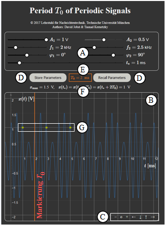
(A) Parametereingabe per Slider
(B) Bereich der graphischen Darstellung
(C) Variationsmöglichkeit für die graphische Darstellung
(D) Abspeichern und Zurückholen von Parametersätzen
(E) Numerikausgabe des Hauptergebnisses T0; graphische Verdeutlichung durch rote Linie
(F) Ausgabe von xmax und der Signalwerte x(t∗)=x(t∗+T0)=x(t∗+2T0)
(G) Darstellung der Signalwerte x(t∗)=x(t∗+T0)=x(t∗+2T0) durch grüne Punkte
(H) Einstellung der Zeit t∗ für die Signalwerte x(t∗)=x(t∗+T0)=x(t∗+2T0)
Details zum obigen Punkt (C)
(*) Zoom–Funktionen „+” (Vergrößern), „−” (Verkleinern) und o (Zurücksetzen)
(*) Verschieben mit „←” (Ausschnitt nach links, Ordinate nach rechts), „↑” „↓” und „→”
Andere Möglichkeiten:
(*) Gedrückte Shifttaste und Scrollen: Zoomen im Koordinatensystem,
(*) Gedrückte Shifttaste und linke Maustaste: Verschieben des Koordinatensystems.
Über die Autoren
Dieses interaktive Berechnungstool wurde am Lehrstuhl für Nachrichtentechnik der Technischen Universität München konzipiert und realisiert.
- Die erste Version wurde 2005 von Bettina Hirner im Rahmen ihrer Diplomarbeit mit „FlashMX–Actionscript” erstellt (Betreuer: Günter Söder ).
- 2018 wurde dieses Programm von Jimmy He im Rahmen seiner Bachelorarbeit (Betreuer: Tasnád Kernetzky) auf „HTML5” umgesetzt und neu gestaltet.
