Exercise 2.8: COST Delay Models

COST delay models

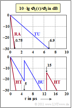
On the right, four delay power density spectra are plotted logarithmically as a function of the delay time $\tau$

$10 \cdot {\rm lg}\hspace{0.15cm} ({{\it \Phi}_{\rm V}(\tau)}/{\it \Phi}_{\rm 0}) \hspace{0.05cm},$

Here the abbreviation $\phi_0 = \phi_{\rm V}(\tau = 0)$ is used. These are the so-called COST–delay models.

The upper sketch contains the two profiles ${\rm RA}$ (Rural Area) and ${\rm TU}$ (Typical Urban). Both of these are exponential:

${{\it \Phi}_{\rm V}(\tau)}/{\it \Phi}_{\rm 0} = {\rm e}^{ -\tau / \tau_0} \hspace{0.05cm}.$

The value of the parameter $\tau_0$ (time constant of the ACF) should be determined from the graphic in subtask (1). Note the specified values of $\tau_{-30}$ for ${\it \Phi}_{\rm V}(\tau_{-30})=-30 \ \rm dB$ :

${\rm RA}\text{:}\hspace{0.15cm}\tau_{-30} = 0.75\,{\rm µ s} \hspace{0.05cm},\hspace{0.2cm} {\rm TU}\text{:}\hspace{0.15cm}\tau_{-30} = 6.9\,{\rm µ s} \hspace{0.05cm}.$

The lower graph applies to less favourable conditions in

urban areas (Bad Urban, ${\rm BU}$ ):

${{\it \Phi}_{\rm V}(\tau)}/{{\it \Phi}_{\rm 0}} = \left\{ \begin{array}{c} {\rm e}^{ -\tau / \tau_0} \\ 0.5 \cdot {\rm e}^{ (5\,{\rm \mu s}-\tau) / \tau_0} \end{array} \right.\quad \begin{array}{*{1}c} \hspace{-0.55cm} {\rm if}\hspace{0.15cm}0 < \tau < 5\,{\rm µ s}\hspace{0.05cm},\hspace{0.15cm}\tau_0 = 1\,{\rm µ s} \hspace{0.05cm}, \\ \hspace{-0.15cm} {\,\, \,\, \rm if}\hspace{0.15cm}5\,{\rm µ s} < \tau < 10\,{\rm µ s}\hspace{0.05cm},\hspace{0.15cm}\tau_0 = 1\,{\rm µ s} \hspace{0.05cm}, \end{array}$

in rural areas (Hilly Terrain, ${\rm HT}$ ):

${{\it \Phi}_{\rm V}(\tau)}/{{\it \Phi}_{\rm 0}} = \left\{ \begin{array}{c} {\rm e}^{ -\tau / \tau_0} \\ {0.04 \cdot \rm e}^{ (15\,{\rm \mu s}-\tau) / \tau_0} \end{array} \right.\quad \begin{array}{*{1}c} \hspace{-0.55cm} {\rm if}\hspace{0.15cm}0 < \tau < 2\,{\rm µ s}\hspace{0.05cm},\hspace{0.15cm}\tau_0 = 0.286\,{\rm µ s} \hspace{0.05cm}, \\ \hspace{-0.35cm} {\rm if}\hspace{0.15cm}15\,{\rm µ s} < \tau < 20\,{\rm µ s}\hspace{0.05cm},\hspace{0.15cm}\tau_0 = 1\,{\rm µ s} \hspace{0.05cm}. \end{array}$

For the models ${\rm RA}$ , ${\rm TU}$ and ${\rm BU}$ the following parameters are to be determined:

The delay spread $T_{\rm V}$ is the standard deviation of the delay $\tau$ .
If the delaypower density spectrum ${\it \Phi}_{\rm V}(\tau)$ has an exponential course as with the profiles ${\rm RA}$ and ${\rm TU}$ , then $T_{\rm V} = \tau_0$ , see Exercise 2.7.

The coherence bandwidth $B_{\rm K}$ is the value of $\Delta f$ at which the magnitude of the frequency correlation function $\varphi_{\rm F}(\Delta f)$ has dropped to half its value for the first time. With exponential ${\it \Phi}_{\rm V}(\tau)$ as with ${\rm RA}$ and ${\rm TU}$ the product $T_{\rm V} is \cdot B_{\rm K} \approx 0.276$ , see Exercise 2.7.

Notes:

This task belongs to chapter GWSSUS–Kanalmodell.
The following integrals are given:

$\frac{1}{\tau_0} \cdot \int_{0}^{\infty}\hspace{-0.15cm} {\rm e}^{ -\tau / \tau_0} \hspace{0.15cm}{\rm d} \tau = 1 \hspace{0.05cm},\hspace{0.6cm} \frac{1}{\tau_0} \cdot \int_{0}^{\infty}\hspace{-0.15cm} {\tau} \cdot{\rm e}^{ -\tau / \tau_0}\hspace{0.15cm}{\rm d} \tau = \tau_0 \hspace{0.05cm},\hspace{0.6cm} \frac{1}{\tau_0} \cdot \int_{0}^{\infty} \hspace{-0.15cm}{\tau^2} \cdot{\rm e}^{ -\tau / \tau_0}\hspace{0.15cm}{\rm d} \tau = 2\tau_0^2\hspace{0.05cm}.$

Questionnaire

${\rm RA} \text{:} \ \hspace{0.4cm} \tau_0 \ = \$

$\ \rm µ s$

${\rm TU} \text{:} \ \hspace{0.4cm} \tau_0 \ = \$

$\ \rm µ s$

${\rm RA} \text{:} \ \hspace{0.4cm} T_{\rm V} \ = \$

$\ \rm µ s$

${\rm TU} \text{:} \ \hspace{0.4cm} T_{\rm V} \ = \$

$\ \rm µ s$

${\rm RA} \text{:} \ \hspace{0.4cm} B_{\rm K} \ = \$

$\ \ \rm kHz$

${\rm TU} \text{:} \ \hspace{0.4cm} B_{\rm K} \ = \$

$\ \ \rm kHz$

	Rural Area $({\rm RA})$ .
	Typical urban $({\rm TU})$ .

${\it \Phi}_{\rm V}(\tau = 5.001 \ \rm µ s) \ = \$

$\ \cdot {\it \Phi}_0$

${\it \Phi}_{\rm V}(\tau = 4,999 \ \rm µ s) \ = \$

$\ \cdot {\it \Phi}_0$

$P_1/(P_1 + P_2) \ = \$

$\ \rm \%$

$T_{\rm V} \ = \$

$\ \rm µ s$

Sample solution

Musterlösung

(1) The following property can be seen from the graph:

$10 \cdot {\rm lg}\hspace{0.1cm} (\frac{{\it \Phi}_{\rm V}(\tau_{\rm -30})}{{\it \Phi}_0}) = 10 \cdot {\rm lg}\hspace{0.1cm}\left [{\rm exp}[ -\frac{\tau_{\rm -30}}{ \tau_{\rm 0}}]\right ] \stackrel {!}{=} -30\,{\rm dB}$

$\Rightarrow \hspace{0.3cm} {\rm lg}\hspace{0.1cm}\left [{\rm exp}[ -\frac{\tau_{\rm -30}}{ \tau_{\rm 0}}]\right ] = -3 \hspace{0.3cm}\Rightarrow \hspace{0.3cm} {\rm ln}\hspace{0.1cm}\left [{\rm exp}[ -\frac{\tau_{\rm -30}}{ \tau_{\rm 0}}]\right ] = -3 \cdot {\rm ln}\hspace{0.1cm}(10)\hspace{0.3cm} \Rightarrow \hspace{0.3cm} \tau_{\rm 0} = \frac{\tau_{\rm -30}}{ 3 \cdot {\rm ln}\hspace{0.1cm}(10)}\approx \frac{\tau_{\rm -30}}{ 6.9} \hspace{0.05cm}.$

Here $\tau_{-30}$ denotes the delay that leads to the logarithmic ordinate value $-30 \ \rm dB$ . Thus one obtains

for rural area (RA) with $\tau_{–30} = 0.75 \ \rm µ s$ :

$\tau_{\rm 0} = \frac{0.75\,{\rm \mu s}}{ 6.9} \hspace{0.1cm}\underline {\approx 0.109\,{\rm µ s}} \hspace{0.05cm},$

for urban and suburban areas (Typical Urban, TU) with $\tau_{–30} = 6.9 \ \rm µ s$ :

$\tau_{\rm 0} = \frac{6.9\,{\rm \mu s}}{ 6.9} \hspace{0.1cm}\underline {\approx 1\,{\rm µ s}} \hspace{0.05cm},$

(2) In Exercise 2.7, it was shown that the delay spread is $T_{\rm V} =\tau_0$ when the delay power density spectrum decreases exponentially according to ${\rm e}^{-\tau/\tau_0}$ . Thus the following applies:

for „Rural Area”: $\hspace{0.4cm} T_{\rm V} \ \underline {= 0.109 \ \rm µ s}$ ,
for „Typical Urban”: $\hspace{0.4cm} T_{\rm V} \ \underline {= 1 \ \rm µ s}$ .

(3) In Exercise 2.7 it was also shown that for the coherence bandwidth $B_{\rm K} \approx 0.276/\tau_0$ applies. It follows:

$B_{\rm K} \ \underline {\approx 2500 \ \rm kHz}$ („Rural Area”),
$B_{\rm K} \ \underline {\approx 276 \ \ \rm kHz}$ („Typical Urban”)

(4) The second solution is correct:

Frequency selectivity of the mobile radio channel is present if the signal bandwidth $B_{\rm S}$ is larger than the coherence bandwidth $B_{\rm K}$ (or at least of the same order of magnitude).
The smaller $B_{\rm K}$ is, the more often this happens.

(5) According to the given equation, we have ${\it \Phi}_{\rm V}(\tau = 5.001 \ \rm µ s)/{\it \Phi}_0 \hspace{0.15cm}\underline{\approx0.5}$ .

On the other hand, for slightly smaller $\tau$ (for example $\tau = 4,999 \ \rm µ s$ ) we have approximately

${{\it \Phi}_{\rm V}(\tau = 4.999\,{\rm \mu s})}/{{\it \Phi}_{\rm 0}} = {\rm e}^{ -{4.999\,{\rm µ s}}/{ 1\,{\rm \mu s}}} \approx {\rm e}^{-5} \hspace{0.1cm}\underline {= 0.00674 }\hspace{0.05cm}.$

(6) The power $P_1$ of all signal components with delays between $0$ and $5 \ \mu\rm s$ is:

$P_1 = {\it \Phi}_{\rm 0} \cdot \int_{0}^{5\,{\rm \mu s}} {\rm exp}[ -{\tau}/{ \tau_0}] \hspace{0.15cm}{\rm d} \tau \hspace{0.15cm} \approx \hspace{0.15cm} {\it \Phi}_{\rm 0} \cdot \int_{0}^{\infty} {\rm e}^{ -{\tau}/{ \tau_0}} \hspace{0.15cm}{\rm d} \tau = {\it \Phi}_{\rm 0} \cdot \tau_0 \hspace{0.05cm}.$

The power outside $[0\;\mu \mathrm{s}, 5\;\mu \mathrm{s}]$ is

$P_2 = \frac{{\it \Phi}_{\rm 0}}{2} \cdot \int_{5\,{\rm µ s}}^{\infty} {\rm exp}[ \frac{5\,{\rm µ s} -\tau}{ \tau_0}] \hspace{0.15cm}{\rm d} \tau \hspace{0.15cm} \approx \hspace{0.15cm} \frac{{\it \Phi}_{\rm 0}}{2} \cdot \int_{0}^{\infty} {\rm exp}[ -{\tau}/{ \tau_0}] \hspace{0.15cm}{\rm d} \tau = \frac{{\it \Phi}_{\rm 0} \cdot \tau_0}{2} \hspace{0.05cm}.$

Correspondingly, the percentage of power between $0$ and $5 \ \mu\rm s$ is

Delay power density of the COST profiles

${\rm BU}$ and

${\rm HT}$

$\frac{P_1}{P_1+ P_2} = \frac{2}{3} \hspace{0.15cm}\underline {\approx 66.7\%}\hspace{0.05cm}.$

The figure shows ${\it \Phi}_{\rm V}(\tau)$ in linear scale:

The areas $P_1$ and $P_2$ are labeled.
The left graph is for ${\rm BU}$ , the right graph is for ${\rm HT}$ .
For the latter, the power percentage of all later echoes (later than $15 \ \rm µ s$ ) is only about $12\%$ .

(7) The area of the entire power density spectrum gives $P = 1.5 \cdot \phi_0 \cdot \tau_0$ .

Normalizing ${\it \Phi}_{\rm V}(\tau)$ to this value yields the probability density function $f_{\rm V}(\tau)$ , as shown in the next graph (left diagram).

Delay PDF of profile

${\rm BU}$

With $\tau_0 = 1 \ \ \rm µ s$ and $\tau_5 = 5 \ \ \rm µ s$ , the mean is:

$m_{\rm V}= \int_{0}^{\infty} f_{\rm V}(\tau) \hspace{0.15cm}{\rm d} \tau$

$\Rightarrow \hspace{0.3cm}m_{\rm V}= \frac{2}{3\tau_0} \cdot \int_{0}^{\tau_5} \tau \cdot {\rm e}^{ - {\tau}/{ \tau_0}} \hspace{0.15cm}{\rm d} \tau \ +$

$\hspace{1.7cm}+\ \frac{1}{3\tau_0} \cdot \int_{\tau_5}^{\infty} \tau \cdot {\rm e}^{ (\tau_5 -\tau)/\tau_0}\hspace{0.15cm}{\rm d} \tau \hspace{0.05cm}.$

The first integral is equal to $2\tau_0/3$ according to the provided expression.

With the substitution $\tau' = \tau \, -\tau_5$ you finally obtain using the integral solutions given above:

$m_{\rm V} \hspace{-0.1cm} \ = \ \hspace{-0.1cm} \frac{2\tau_0}{3} + \frac{1}{3\tau_0} \cdot \int_{0}^{\infty} (\tau_5 + \tau') \cdot{\rm e}^{ - {\tau}'/{ \tau_0}} \hspace{0.15cm}{\rm d} \tau ' = \frac{2\tau_0}{3} + \frac{\tau_5}{3\tau_0} \cdot \int_{0}^{\infty} \cdot{\rm e}^{ - {\tau}'/{ \tau_0}} \hspace{0.15cm}{\rm d} \tau ' + \frac{1}{3\tau_0} \cdot \int_{0}^{\infty} \tau' \cdot \cdot{\rm e}^{ - {\tau}'/{ \tau_0}} \hspace{0.15cm}{\rm d} \tau '$

$\Rightarrow \hspace{0.3cm}m_{\rm V}= \frac{2\tau_0}{3} + \frac{\tau_5}{3}+ \frac{\tau_0}{3} = \tau_0 + \frac{\tau_5}{3} \hspace{0.15cm}\underline {\approx 2.667\,{\rm µ s}} \hspace{0.05cm}.$

The variance $\sigma_{\rm V}^2$ is equal to the second moment (mean of the square) of the zero-mean random variable $\theta = \tau \, –m_{\rm V}$ , whose PDF is shown in the right graph
From this $T_{\rm V} = \sigma_{\rm V}$ can be specified.

A second possibility is to first calculate the mean square value of the random variable $\tau$ and from this the variance $\sigma_{\rm V}^2$ using Steiner's theorem.
With the substitutions and approximations already described above, one obtains

$m_{\rm V2} \hspace{-0.1cm} \ \approx \ \hspace{-0.1cm} \frac{2}{3\tau_0} \cdot \int_{0}^{\infty} \tau^2 \cdot {\rm e}^{ - {\tau}/{ \tau_0}} \hspace{0.15cm}{\rm d} \tau + \frac{1}{3\tau_0} \cdot \int_{0}^{\infty} (\tau_5 + \tau')^2 \cdot {\rm e}^{ - {\tau}'/{ \tau_0}} \hspace{0.15cm}{\rm d} \tau '$

$\Rightarrow \hspace{0.3cm}m_{\rm V2} = \frac{2}{3} \cdot \int_{0}^{\infty} \frac{\tau^2}{\tau_0} \cdot {\rm e}^{ - {\tau}/{ \tau_0}} \hspace{0.15cm}{\rm d} \tau + \frac{\tau_5^2}{3} \cdot \int_{0}^{\infty} \frac{1}{\tau_0} \cdot {\rm e}^{ - {\tau}'/{ \tau_0}} \hspace{0.15cm}{\rm d} \tau ' +\frac{2\tau_5}{3} \cdot \int_{0}^{\infty} \frac{\tau '}{\tau_0} \cdot {\rm e}^{ - {\tau}'/{ \tau_0}} \hspace{0.15cm}{\rm d} \tau ' + \frac{1}{3} \cdot \int_{0}^{\infty} \frac{{\tau '}^2}{\tau_0} \cdot {\rm e}^{ - {\tau}'/{ \tau_0}} \hspace{0.15cm}{\rm d} \tau ' \hspace{0.05cm}.$

With the integrals given above, we have

$m_{\rm V2} \approx \frac{2}{3} \cdot 2 \tau_0^2 + \frac{\tau_5^2}{3} \cdot 1 + \frac{2\tau_5}{3} \cdot \tau_0 + \frac{1}{3} \cdot 2 \tau_0^2 = 2 \tau_0^2 + \frac{\tau_5^2}{3} + \frac{2 \cdot \tau_0 \cdot \tau_5}{3}$

$\Rightarrow \hspace{0.3cm} \sigma_{\rm V}^2 \hspace{-0.1cm} \ = \ \hspace{-0.1cm} m_{\rm V2} - m_{\rm V}^2 = 2 \tau_0^2 + \frac{\tau_5^2}{3} + \frac{2 \cdot \tau_0 \cdot \tau_5}{3} - (\tau_0 + \frac{\tau_5}{3})^2 =\tau_0^2 + \frac{2\tau_5^2}{9} = (1\,{\rm µ s})^2 + \frac{2\cdot (5\,{\rm µ s})^2}{9} = 6.55\,({\rm µ s})^2$

$\Rightarrow \hspace{0.3cm} T_{\rm V} = \sigma_{\rm V} \hspace{0.15cm}\underline {\approx 2.56\,{\rm µ s}}\hspace{0.05cm}.$

The above graph shows the parameters $T_{\rm V}$ and $\sigma_{\rm V}$ .